Bubbling is a mass transfer process between gas and liquid, commonly found in various industrial applications such as beverage carbonation and photobioreactors. Even the act of aerating a fish tank at home falls under this phenomenon. In this article, we will detail how to simulate the carbonation process, a type of bubbling phenomenon, using COMSOL Multiphysics® software.
What is Bubbling?
Bubbling is the process of introducing gas into a liquid to create bubbles, thereby dissolving the gas in the liquid or stripping the liquid of certain dissolved components. As mentioned, this process facilitates mass transfer from gas to liquid or from liquid to gas. An example of this is the deoxygenation process, in which nitrogen gas bubbles pass through the liquid, displacing or removing oxygen and other dissolved gases. Another example is dissolution, where gas dissolves in liquid. The dissolved substances can further react with other components in the liquid, altering the chemical composition of the liquid. Carbonation and aeration are common examples of this bubbling/dissolution phenomenon.
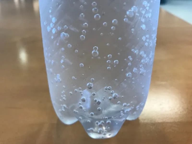
The bubbles generated by the carbonation process in a bottle of soda
When we open a bottle of soda, sparkling water, or any carbonated beverage, we hear a “hissing” sound due to the release of pressure and the buoyancy that causes carbon dioxide bubbles to rise. However, before we open the cap, carbon dioxide is dissolved in the beverage (CO2(aq)). This dissolution occurs as carbon dioxide bubbles (typically under supersaturated high pressure) pass through the liquid. As the carbon dioxide bubbles move through the beverage, gas is transferred to the liquid through the surface of the bubbles, and the dissolved carbon dioxide reacts with water to form carbonic acid. This entire process is known as carbonation.
In this article, we will explore how to simulate the carbonation process through the dissolution of carbon dioxide in water—essentially creating virtual carbonated water.
A Close-Up Look at Carbonation
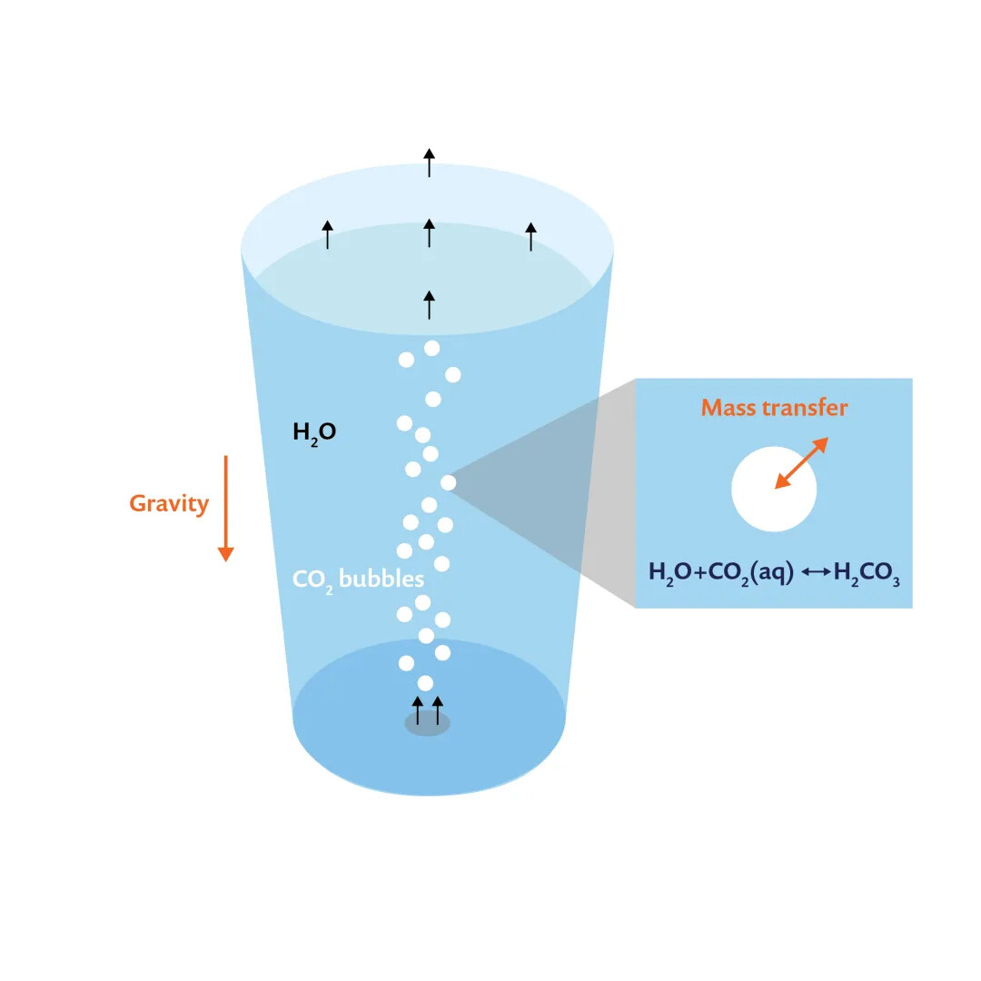
As shown in the figure below, carbon dioxide is introduced from the bottom of a glass of water. Due to buoyancy, carbon dioxide bubbles rise and travel through the water, transferring mass and momentum, ultimately escaping through the surface. It is important to note that the dissolved carbon dioxide reacts with water to form carbonic acid. Therefore, to simulate and understand the carbonation process in a glass, we need to solve the following problems:
- The mass and momentum transfer of water and carbon dioxide bubbles, i.e., multiphase flow.
- The mass transfer of carbon dioxide from the bubbles to the liquid, i.e., dissolution.
- The mass transfer of dissolved carbon dioxide and any subsequent reactions that occur (such as the formation of carbonic acid).
A schematic diagram of carbonation in a glass of water, with carbon dioxide bubbles entering from the bottom
Simulating Bubbling in COMSOL Multiphysics®
Let’s take a look at the interfaces and conditions needed to solve the bubbling problem in COMSOL Multiphysics. As shown in the figure above, this problem is axisymmetric. Therefore, we can use a 2D axisymmetric component to construct the model. Since the bubble volume fraction is less than 1%, the density of carbon dioxide gas can be neglected compared to water, allowing us to use the bubbly flow and laminar flow interfaces to simulate multiphase flow. When the bubble volume fraction is less than 1%, particle tracking can also be used to solve for the transport of bubbles. However, note that bubbly flow can be used to simulate systems where the bubble volume fraction is greater than 1% (around 10% or less).
Additionally, the Reynolds number calculated based on bubble velocity is below 2000, which indicates laminar flow for internal flows.
You can learn about the advantages and disadvantages of different types of multiphase flow interfaces, as well as their basic assumptions, by reading the articles in the COMSOL® software documentation.
The bubbly flow and laminar flow interfaces can not only solve for velocity, pressure, and effective gas density but also compute the bubble number density and the associated interfacial area (when the option to solve for interfacial area is selected in the settings). Therefore, we can use the double-film theory to calculate the mass transfer between bubbles and the liquid, which will be discussed later.
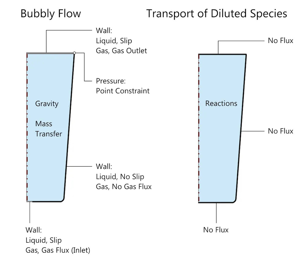
A schematic diagram of the problem setup in COMSOL Multiphysics, showing the boundary and domain conditions related to the bubbly flow and dilute mass transfer interfaces. The mass transfer of carbon dioxide is specified through reaction conditions, while the carbonation reaction is specified through equilibrium reaction conditions; both are represented as reactions in the schematic. Note: Default domain conditions, such as fluid properties, transfer properties, and initial values, are not indicated.
Please note that when simulating fluid flow, we assume that the deformation of the free surface (i.e., the water surface) can be neglected. However, since this is a free surface, a slip wall condition is chosen at the boundary, as shown in the figure above. This condition allows tangential movement of the water while limiting the normal velocity to zero. The gas inlet and outlet conditions are specified under the wall boundary conditions of this interface. (You can find more detailed information about this process in the article on simulating bubbly flow in beer.) To maintain consistency, the inlet gas flux increases from zero to the desired value, which is a time-varying load method and a good practice.
The transfer of aqueous carbon dioxide and carbonic acid resulting from the equilibrium reaction between carbon dioxide and water is simulated using the dilute mass transfer interface, which addresses the concentration of aqueous carbon dioxide and carbonic acid. Note that in this example, we only consider the reaction that generates carbonic acid. The relevant boundary conditions for bubbly flow (bf) and dilute mass transfer (tds) are shown in the figure above.
The mass transfer of carbon dioxide from the bubbles to the liquid is simulated through the mass transfer conditions of the bubbly flow interface. In this example, we use the double-film theory option, which utilizes Henry’s law to calculate the mass transfer required from gas to liquid. This is given by the following equation:
![]()
Where:
k is the mass transfer coefficient that must be specified, derived from experiments or literature.
c is the concentration of the solute; in this case, it is the concentration of aqueous carbon dioxide c_CO2 , calculated using the dilute mass transfer interface.
M is the molecular weight of the gas (carbon dioxide).
a is the interfacial area per unit volume, calculated through the bubbly flow interface.
c* is the equilibrium concentration calculated according to Henry’s law,
![]()
where:
p is the relative pressure calculated through the bubbly flow interface.
pref is the reference pressure specified in the bubbly flow interface.
H is the Henry’s constant, derived from experiments or literature.
The mass transfer from gas to liquid is the source of aqueous carbon dioxide, analyzed through the reaction term in the dilute mass transfer interface, as shown below. In addition to the coupling between the dilute mass transfer and bubbly flow interfaces, the liquid phase velocity calculated through the bubbly flow interface is conveyed in the transfer properties domain settings of the dilute mass transfer interface, which explains the convective transfer of aqueous carbon dioxide.
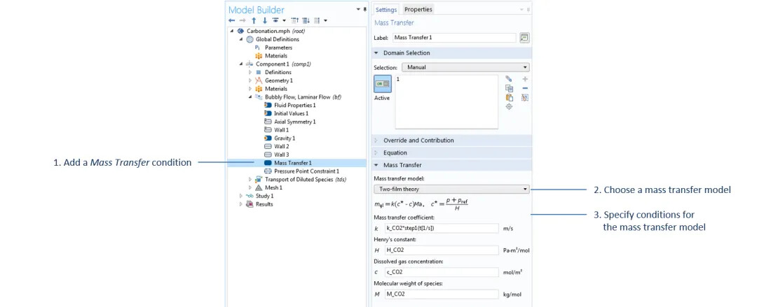
The settings for the mass transfer conditions in the bubbly flow interface. Except for c_CO2, which is the concentration of carbon dioxide calculated in the dilute mass transfer interface, all parameters in this domain feature are defined under the parameter node.
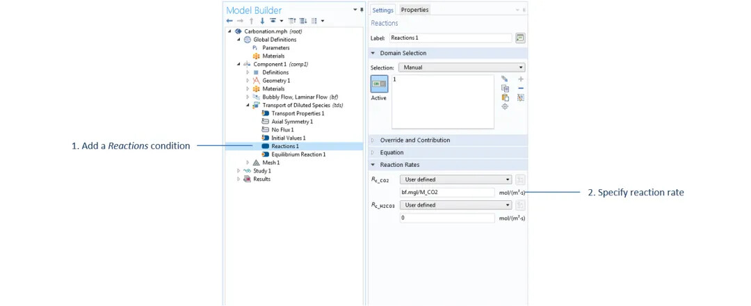
The settings for the reaction term in the dilute mass transfer interface, where the mass transfer value bf.mgl is calculated in the bubbly flow interface and transferred as a source/sink term in the dilute mass transfer interface.
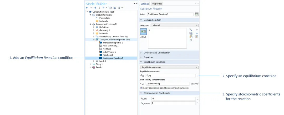
The settings used to specify the equilibrium reaction H2O + CO2 (aq) ↔ H2CO3, with water acting as the solvent in the dilute mass transfer interface, where K_eq is defined under the parameter node.
Simulation Results of the Bubbling Process
The relevant input information for the mass transfer of carbon dioxide and the diffusion of aqueous carbon dioxide is derived from the literature.
By comparing the plots at t=0s and t=10s shown below, it is clear that the carbon dioxide bubbles (quantified by the gas volume fraction) begin to rise in the water, imparting momentum to the water and eventually escaping through the surface. However, since the water does not flow out through the surface but circulates within the glass, this results in the observed vortices in the figure below. Mass transfer occurs in regions where the gas volume fraction is non-zero, so the initial concentration of aqueous carbon dioxide is closely related to the gas volume fraction. As aqueous carbon dioxide is transferred to the rest of the glass through convection and diffusion, it can be seen from comparing the velocity, streamlines, and surface plots of aqueous carbon dioxide concentration that convective transfer is dominant.
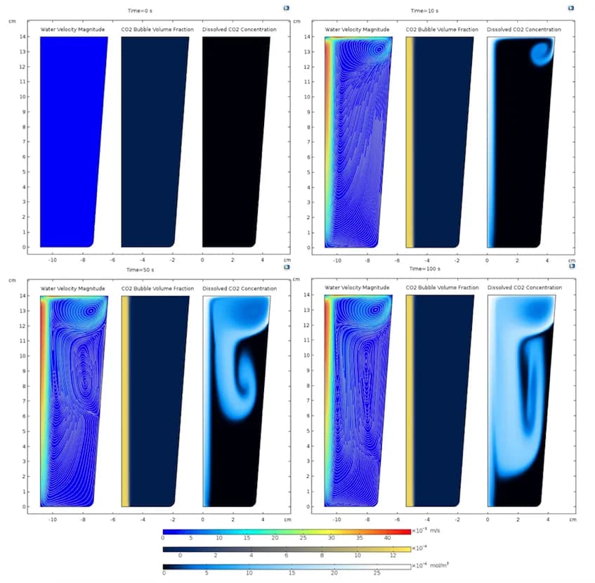
At t={0,10,50,100}s, the velocity magnitude of the water and the streamlines (left), the volume fraction of carbon dioxide bubbles (middle), and the concentration of aqueous carbon dioxide (right)
In COMSOL Multiphysics, we can also create and export animations of the above plots, which helps to better observe the formation of vortices, their evolution over time, and the transfer of dilute substances.
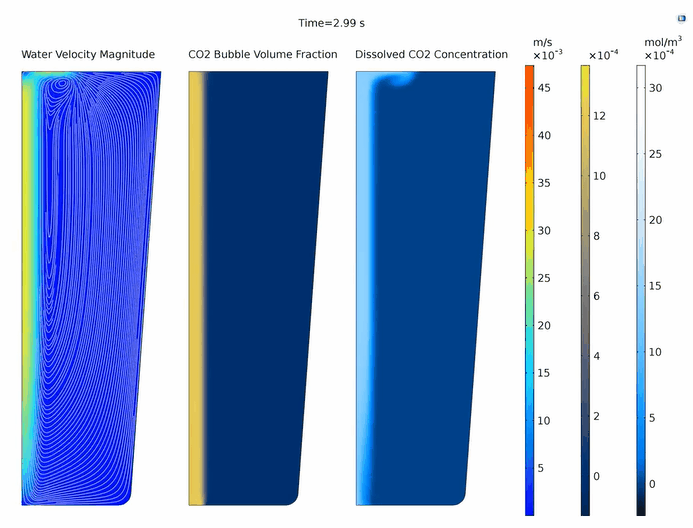
The evolution of the velocity magnitude of the water and the streamlines (left), the volume fraction of carbon dioxide bubbles (middle), and the concentration of aqueous carbon dioxide (right).
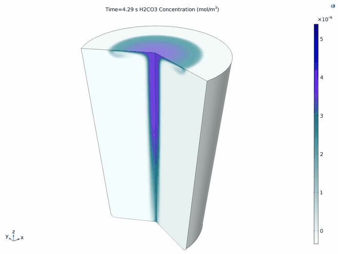
Since this is a 2D axisymmetric simulation, COMSOL Multiphysics automatically creates a 3D dataset, marking a transformation in the computation of 2D datasets. Therefore, we can create a 3D animation showing the evolution of carbonic acid over time, where the generation and transfer of carbonic acid are closely related to the transfer of aqueous carbon dioxide.